(KANs part 1) An introduction to B-splines
In this blog series, I'll be going through the technical details involved in understanding Kolmogorov-Arnold Networks - a new type of machine learning architecture which has gotten significant attention lately due to it's several advantages over MLPs(Multi Layer Perceptrons), such as interpretability and avoiding catastrophic forgetting to name a few.
Table of Contents:
In part one of this series, let's build our understanding from the ground up, starting from polynomial interpolation and progressing to B-splines, the workhorse of the Kolmogorov-Arnold Network (KAN). B-splines are used in KANs to learn activation functions. Let's start with simple polynomial interpolation.
Polynomial interpolation #
The goal of polynomial interpolation is to find the coefficients of a polynomial , such that it passes through your data points.
For example, if we had 4 data points , we could fit a cubic polynomial through it by solving for in the following system of equations:
Here's an example of the fit with some toy data:
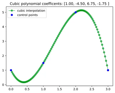
You'd need a polynomial of degree , to pass through data points. A higher polynomial degree would imply non-unique solutions, and a lower polynomial degree would imply non-existence of a solution (unless in special cases). Let's see what a higher order polynomial fit looks like:
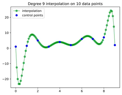
This interpolation looks reasonable in the middle, but what's going on at the edges? Those jumps look a bit too extreme. Well, we've encountered the well-known Runge's phenomenon, where higher degree polynomials oscillate at the edges. This leads us to one of the many motivations behind using splines for interpolation.
Splines #
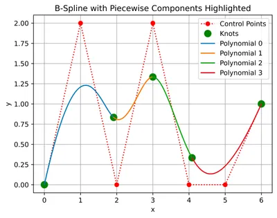
We can think of splines as combining many low-order polynomials in order to create a more complex, smooth curve. These low order polynomials are often cubic, since cubic polynomials offer a good tradeoff between expressivity and complexity. Splines have many varieties, mostly involving different ways these individual polynomial pieces can be joined, such that they smoothly flow from one to the other.
Splines can be either interpolating (passing through all the data points, also called control points), or approximating (not necessarily passing though the data points).
Let's first see how splines can be better than polynomial interpolation (the same points below apply for approximation tasks as well):
| Feature | Polynomial Interpolation | Spline Interpolation |
|---|---|---|
| Degree | Single polynomial of degree for points | Lower-degree polynomials (typically cubic) for each interval |
| Continuity | Ensures smoothness over entire range | Ensures smoothness at the knots (joining points) |
| Local Control | No local control, changing one point affects the entire polynomial | Local control, changing one point affects only the nearby intervals. This is a desirable feature for interpolation tasks. B-splines, among other splines, have this property. |
| Runge's Phenomenon | Susceptible to Runge's phenomenon (oscillations at the edge) | Avoids Runge's phenomenon |
| Efficiency | Computationally intensive for large datasets | More efficient for large datasets due to local computation |
| Flexibility | Less flexible for complex shapes | More flexible |
The overall geometric shape of the spline is determined by user-specified control points. The individual polynomial pieces are connected at points called knots. The knots determine how and where the spline is split up into smaller polynomials. The knots can be any increasing sequence of numbers. In some splines, like the Catmull-Rom spline, the knots can be the same as the control points. However, this is not always the case. For example, in approximating B-splines, since the final curve does not necessarily pass through the control points, the piecewise polynomials are not joint at the control points but at some other approximated location. Hence we can see that the knots are not the same as the control points. We will look at different types of knot vector constructions later in this article.
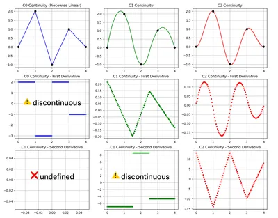
Continuity #
Continuity (or "smoothness") is a measure of how smoothly one polynomial connects to the other. When thinking of smoothness, one can naturally think of having a continuous rate of change, and this is indeed a form of continuity, called continuity, where the first derivative is continuous at the joins.
There can be some physical intuition here, because if you imagine a tangent vector moving along the spline, continuity implies it moving at a continuous speed (the first derivative of distance with respect to time). Notably, there is no abrupt change of speed at the join in particular, because before the join, we're on a smooth polynomial anyway. continuity would imply no sudden change of acceleration at the join, and so on. The lovely video by Freya Holmér on the continuity of splines beautifully explains and animates continuity measures, including other ones, like geometric continuity which we won't get into here.
In general, continuity means that the derivative is continuous at the joins, and implies that the lower ( ) derivatives also exist and are continuous. A higher gives us a smoother curve.
Basis functions #
I want to touch on the intuition behind basis functions before we jump into B-splines. We mentioned that control points affect the geometric shape of the curve, but how? They do this by using their corresponding basis function. The influence or "pull" that a control point has is determined by it's basis function, and there are as many basis functions as there are control points. A widely spread out basis function for a specific control point would imply that moving the control point can affect a larger part of the curve. The animation below represents this quite well.
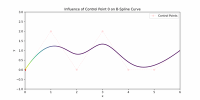
I found that the Scipy docs on B spline basis functions are also a useful read!
B-splines #
B-splines are continuous and have local control. In addition, the control points defining the spline so not need to be uniformly spaced, making it flexible and useful for many real world use cases.
In cubic B-splines, each piecewise polynomial is expressed as
where represent the 4 control points that are needed to define a cubic polynomial (recall from the polynomial interpolation section, that a polynomial of degree needs points to define it). This cubic polynomial piece of the spline is a parametric curve, where is a parameter that goes between and . The final curve can also be represented in cartesian coordinates as , where and can be computed by substituting the and coordinates of the control points into the above equation.
Expanding the equation, we get our basis functions. The matrix of numbers in the equation from which we expand might look arbitrary, but these values can actually be solved for. We solve for them by specifying our constraints for the B-spline, namely continuity and requiring that the basis functions sum up to one.
Plotting the functions influencing each control point, we can see the cubic B-spline basis functions look like this (graph on desmos):
![Fig 6: Cubic spline basis functions for 4 control points, for t ∈ [0,1]. In the graph, the variable x refers to t.](/img/ng4d-Ujgpf-400.webp)
These represent the influences of the 4 control points throughout one cubic piece of a spline. You can see the influence of the control points on the whole spline in the animated figure in the basis functions section.
Cox-de Boor recursion formula #
The Cox-de Boor formula tells us how to calculate the basis functions of a B-spline. The cool part about this algorithm is that it is trivial to use this to calculate the B-spline basis functions in higher dimensions. Let be the control point vector, and be the corresponding basis function of a B-spline with degree . We have control points and basis functions (going from ). Our spline will be a linear combination of these:
The Cox-de Boor algorithm is recursive, with a base case and a recursive step. It allows us to express higher-degree basis functions in terms of lower degree ones. Let be the knot position (the knots are defined in parameter space and are thus scalar), and be domain of the function, spanning the domain of the control points provided. The base case for degree is
This is telling us that the base case is just a step function, which is 1 in the knot interval and zero elsewhere. The recursive step is:
The basis function for higher degrees is expressed as a weighted combination of two lower-degree basis functions, which I've highlighted in red. It is nonzero in the interval . Their scaling factors ensure a smooth transition from one to the other.
Things can be easier to understand with some code. Here's an example implementation!
def cox_de_boor(u, i, k, knots):
    """
    u : x value of the point to be evaluated in the input domain
    i : index of the basis function to compute
    k : degree of the spline
    knots : values in the parameter domain that divide the spline into pieces

    returns -> a scalar value that calculates the influence of the i'th basis function on the point u in the input domain.
    """
    if k == 0:
        return 1.0 if knots[i] <= u < knots[i + 1] else 0.0
    left_term = 0.0
    right_term = 0.0
    if knots[i + k] != knots[i]:
        left_term = (
            (u - knots[i]) / (knots[i + k] - knots[i]) * cox_de_boor(u, i, k - 1, knots)
        )
    if knots[i + k + 1] != knots[i + 1]:
        right_term = (
            (knots[i + k + 1] - u)
            / (knots[i + k + 1] - knots[i + 1])
            * cox_de_boor(u, i + 1, k - 1, knots)
        )
    return left_term + right_term
Fitting a B-spline with code #
Let's fit a B-spline to some data. In the process, we'll play with different configurations of the knot vector: uniform, open uniform and non-uniform.
import numpy as np
import matplotlib.pyplot as plt

def evaluate_spline(control_points, knots, evaluation_interval):
    # Calculate the basis functions
    basis_functions = np.zeros((len(u_values), num_basis_functions))
    for i in range(num_basis_functions):
        basis_functions[:, i] = [cox_de_boor(u, i, degree, knots) for u in u_values]
    # basis_functions[-1, -1] = 1

    # Construct the B-spline curve - a linear combination of basis functions weighted by the control points
    curve = np.zeros((len(evaluation_interval), 2))
    for i in range(num_basis_functions):
        curve += basis_functions[:, i].reshape(-1, 1) * control_points[i]

    fig, axs = plt.subplots(2, 1, figsize=(5, 5), dpi=1200)

    # Plot the basis functions
    for i in range(num_basis_functions):
        axs[0].plot(u_values, basis_functions[:, i], label=f"B{i}")
    axs[0].set_xlabel("u")
    axs[0].set_ylabel("Basis Function Value")
    axs[0].set_title("Cubic B-Spline Basis Functions")
    axs[0].legend()
    axs[0].grid(True)
    # Plot the B-spline curve and control points
    axs[1].plot(curve[:, 0], curve[:, 1], label="B-Spline Curve")
    axs[1].plot(
        control_points[:, 0], control_points[:, 1], "ro--", label="Control Points"
    )
    axs[1].set_xlabel("x")
    axs[1].set_ylabel("y")
    axs[1].legend()
    axs[1].set_title("Cubic B-Spline Curve")
    axs[1].grid(True)

    # Show the plot
    plt.tight_layout()
    plt.show()
Uniform knot vectors #
Recall that in a cubic spline, each basis function is nonzero only in a fixed interval, not the whole range of the spline (the so called compact support, important for local control). For a cubic B-spline, this interval spans knots. This is the reason why B-splines have more knots than control points. Specifically, if we have control points (from ), then we'll have knots, where is the spline degree.
Another interesting fact is that the shape of the resulting basis functions are independant of any scaling/translating we might do to the knot vector, it purely depends on the relative spacing between the knots.
A uniform knot vector has equal spacing between all the knots. In the code and figure below, you'll notice that the spline is only evaluated between the knots and . This is because at the ends, the basis functions do not have enough support and do not sum up to one. As a result, the curve starts deviating from the control points in unexpected ways.
control_points = np.array([[0, 0], [1, 2], [2, 0], [3, 2], [4, 0], [5, 0], [6, 1]])
# uniform
knots = np.arange(n + degree + 2)
degree = 3
u_values = np.linspace(knots[degree], knots[-degree - 1], 100)
evaluate_spline(control_points, knots, u_values)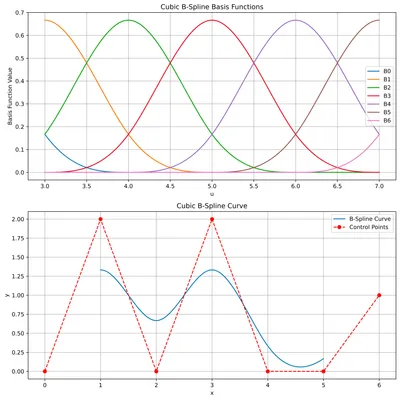
Open uniform knot vectors #
As we move into unequal knot spacing territory, the splines are not necessarily continuous everywhere.
To make the spline also go through the first and last points, we can modify our uniform knot vector such that the first and last point have full influence (1) at the beggining and end of the spline.
This is done via "knot clamping", where the first and last values of a uniform knot vector are just repeated. Note again, that only the relative spacing between the knots and not the knot values itself influence the shape of the basis functions.
If knot values are bought closer, this brings the curve closer to the associated control point. If the values are repeated, for each repetition, the degree of continuity is reduced for the knot value. In this case, repeating the value more times makes the curve discontinuous at the start and the end (going from ). In addition, all the local influence to the spline is attributed to these points, as seen in Fig 8.
control_points = np.array([[0, 0], [1, 2], [2, 0], [3, 2], [4, 0], [5, 0], [6, 1]])
# open uniform
knots = np.array([0, 0, 0, 0, 1, 2, 3, 4, 4, 4, 4])
degree = 3
u_values = np.linspace(knots[degree], knots[-degree - 1], 100)
evaluate_spline(control_points, knots, u_values)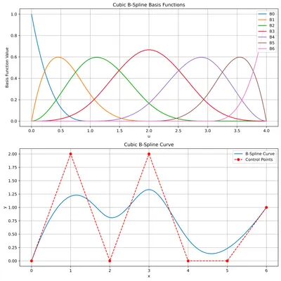
Non-uniform knot vectors #
Here, unequal spacing can be done anywhere, not just at the ends. For example, if we want a sharp bend at the center, we could make it continuous (discontinuous first derivative) by repeating the central knot value more times. This is useful in cases where sharp changes are desired.
In this example, we clamp the ends and introduce continuity in the center:
control_points = np.array([[0, 0], [1, 2], [2, 0], [3, 2], [4, 0], [5, 0], [6, 1]])
# non-uniform
knots = np.array([0, 0, 0, 0, 2, 2, 2, 4, 4, 4, 4])
degree = 3
u_values = np.linspace(knots[degree], knots[-degree - 1], 1000)
evaluate_spline(control_points, knots, u_values)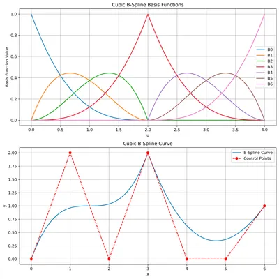
Closing #
Hope you enjoyed this article about B-splines! Do check out the amazing material I referred to in the References section. I could not find a resource quite like this one on the internet, so I hope my exploration can be a useful starting point for you.
If you have any feedback, leave them with the blog title on Issues · RohanGautam/rohangautam.github.io. We started from polynomial interpolation, talked about splines, and took a look at the construction of B-splines with different knot setups in this post. I plan on following this up with more on how they are used in KANs, touching on grid extension, stacking splines and more. Follow me on Twitter/X to hear about it when it's done.
Citation #
BibTeX:
@article{rohan2024bspline,
  title   = "(KANs part 1) An introduction to B-splines",
  author  = "Gautam, Rohan",
  journal = "rohangautam.github.io",
  year    = "2024",
  month   = "Jun",
  url     = "https://rohangautam.github.io/blog/b_spline_intro/"
}
References #
- pg2455/KAN-Tutorial: Understanding Kolmogorov-Arnold Networks: A Tutorial Series on KAN using Toy Examples (github.com)
- Splines in 5 minutes: Part 1 -- cubic curves (youtube.com) a three part series
- The Continuity of Splines (youtube.com)
- B-spline - Wikipedia
- B-splines (cam.ac.uk)
- Previous: Estimating π by throwing needles
- Next: SDFs and Fast sweeping in JAX