Gaussian integration is cool

• 08 June 2025
• simulation,
• numerical_techniques

Numerical integration techniques are often used in a variety of domains where exact solutions are not available. In this blog, we'll look at a numerical integration technique called gaussian quadrature, specifically chebyshev-gauss quadrature. This is applicable for evaluating definite integrals over $[-1,1]$ and with a special functional form - we'll also look into how we can tweak an generic function over an arbitrary interval to fit this form.

Gaussian quadrature #

At it's core, gaussian quadrature gives us a way to evaluate a definite integral of a function by using the function evaluations at special points called nodes, the exact location of which can vary depending on the technique used - we'll look at a specific example using chebyshev nodes later on. Here's the basic idea for a definite integral over $[-1,1]$, we'll extend this to an arbitrary interval $[a,b]$ later on. An integral of $f$ can be expressed as a weighted sum of $f$ evaluated at $n$ nodes :

$\int_{-1}^{1}f(x)dx = \sum_{i=1}^{n}{w(x_i)f(x_i)}$

Elementary integration techniques work by approximating the function $f$ with a polynomial. If we sample the function at n points, we can fit a polynomial of degree n-1, and integrate that to get the approximation. Basically this means that with n nodes, we can integrate polynomials with degree n-1. In contrast, Gaussian quadrature can estimate a polynomial of order 2n-1 with n nodes and another set of n weights. The weights are easily determined based on the specific technique, but now you need roughly half the number of function evaluations for an accurate integral approximation.

This is a great improvement in terms of numerical accuracy for the accuracy you get per function evaluation at a node. Gaussian quadrature does this by carefully selecting nodes - the nodes are given by the roots of an orthogonal polynomial function. These orthogonal polynomials act as a "basis", just like spline coefficients do for spline fitting (with the difference of global instead of local support). By the definition of orthogonality, these have an inner product (dot product in euclidean space) of zero with each other, and that simplifies the necessary calculations (proof)^[1] .

Chebyshev-Gauss quadrature #

This flavour of gaussian quadrature involves using the roots of chebyshev polynomials to decide which nodes to evaluate the function for integration at. The roots of this polynomial are concentrated more on the edges of the domain helping counter oscillation at the boundaries when fitting polynomials (Runge's phenomenon). Additionally, the weights w are fixed at $\pi/n$ , where n is the number of nodes - a parameter you choose.

This specific form of gaussian quadrature can integrate functions of this form:

$\int_{-1}^{1}\frac{f(x)}{\sqrt{1-x^2}}dx = \sum_{i=1}^{n}{w_if(x_i)}$

where the nodes $x_i$ are chebyshev nodes of the first order, and $w_i$ is constant :

$\begin{array}{lcl} x_i=\cos({\pi(i+0.5)}/{n})\\ w_i=\pi/n \end{array}$

Let's extend this to arbitrary intervals and functional forms.

Extending to general functions and integration intervals #

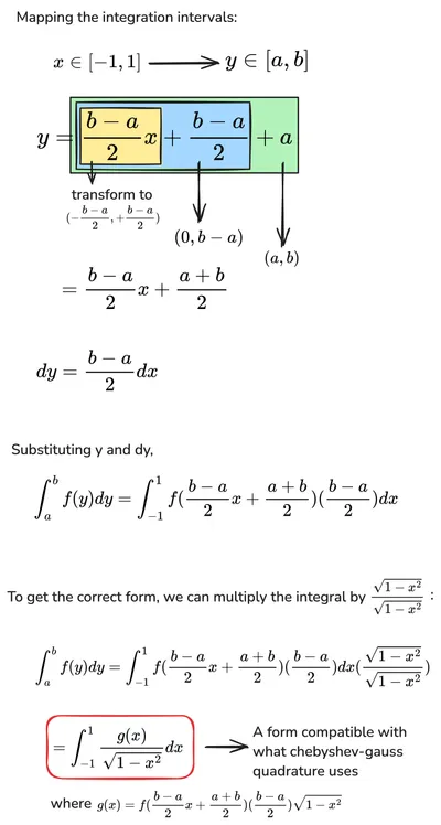
Basically, our goal is to make Chebyshev-Gauss quadrature it work for the following integral:

$\int_{a}^{b}f(y)dy$

Note that we don't have $\sqrt{1-x^2}$ in the denominator and the intervals of integration are arbitrary. We'll take this general representation and massage it into the form that the numerical integration expects. I'm using $y$ as the variable here. Figure 3 shows this transformation.

Let's see it in action! #

This is my first time trying a marimo notebook. It reminds me of what pluto is for julia - in the sense it's a reactive notebook, but with a lot of other cool features. The result is a highly interactive, embeddable notebook experience that's great for short blogs like this - and runs in the browser with WASM! I've also made the code available as a gist here.

You can play around with the slider which controls the number of nodes used for integration. Changing it effects all other conencted cells, allowing you to compare the accuracy of the two integral approximation techniques. For this example, we integrate $\sin(x)$ from $0$ to $\pi$.

Parting thoughts #

This is a cool numerical integration technique I thought I'd share. I used it in my library for estimating rates of sea level change - check out EIV_IGP_jax. A gaussian process prior is fit with MCMC on the rate of sea level change, which is then compared to the observation (heights and times) of sea level proxies by integrating the rate process. The integration step uses chebyshev-gauss quadrature. The specific implementation of the quadrature in that project makes heavy use of broadcasting operations for efficient vectorisation of these calculations over a grid. That was a fun project too, and maybe can be a blog for another day.

• Previous: SDFs and Fast sweeping in JAX