SDFs and Fast sweeping in JAX

• 04 May 2025
• jax,
• simulation

This is going to be a fun blog - we'll explore the intuition behind level sets, the Eikonal equation, and implement a speedy algorithm for solving this equation, called the fast sweeping method, in JAX.

I was recently researching a problem that involved interface evolution over time. Our interface was represented by a set of points. To evolve this interface along its normal direction, we were approximating the normals for these points, extending the points along the normal direction, then resampling them to maintain point density - since, if the shape had expanded, the point density would have decreased. This method of propagating interfaces, involving tracking particles on the front as it evolves, is known as Lagrangian front evolution, and comes with a host of problems, such as resampling issues, handling particles that "grow into" a surface, etc.

The level set method and the eikonal equation #

An alternative view of propagating interfaces was provided by Sethian and Osher, where they developed the level set theory of propagating interfaces. The key difference is that this is an Eulerian approach - the interface is tracked implicitly on a fixed grid, not as particles on the surface as before. In the level set technique, this implicit representation of the surface is the zero level set of a function. What that means, is that you'll have some function defined on your grid, and the grid points where this function is zero will represent your surface. This function (let's call it $\phi$) is the level set function, and is a higher order function, with x,y (in 2D) and time as it's inputs. $\phi(x_{grid}, y_{grid}, t=k)$ gives you the zero level set at time $k$, describing your interface. It is this function that we want to learn/approximate. Most of the time, the level set function at a specific point in time is the signed distance function.

The initial value problem defined by the level set theory allows for both positive and negative propagation speeds along the normal. In fact, for most complex problems involving the level set technique, designing an appropriate propagation speed is crucial, as mentioned in Sethian's book. In this blog, we'll consider a simpler case, where the propagation speed is only positive - this is the case in several important applications.

The equation we'll be looking at solutions of is known as the Eikonal equation, and it looks like this:

$|\nabla T| F=1$

This is a hyperbolic PDE. If you imagine light from a flame propagating from a point, then $T$ is the arrival time of the flame at a specific grid point. $F$ is the propagation speed, and $\nabla$ is the gradient operator. Both $T$ and $F$ are functions which take in a spatial vector $x$. You can imagine this being extremely useful in modelling wavefronts - for example, in the Huygens principle, where each point on the new wave acts as a source of secondary wavelets, and the front is a envelope of the outer parts of these wavelets. It's also used in seismic studies - as wave propagation translates directly to these, as well as shortest path problems, medical imaging and so on. More recently, it's also been used to construct signed distance functions (SDFs) of arbitrary geometry, a representation being increasingly used in implicit representations of 3D surfaces in machine learning. For SDFs, $F=1$.

The Eikonal equation can develop shocks and singularities, for example, near obstacles or a self-collapsing curve (see Fig 2). Traditional numerical methods for solving the eikonal equation (discretising the PDE into a system of ODEs defined on a grid, use a numerical integrator like Runge-Kutta to solve the ODEs, and so on) do not handle shocks and singularities well. For example, a classical numerical routine for solving this equation in presence of an obstacle would not give you a signed distance function. For this reason, there are other more efficient handcrafted algorithms we can use.

Fast sweeping method #

The Fast Marching Method (FMM), introduced by Sethian, solves the Eikonal equation in $O(n\log n)$ time ($n$ is the grid size), using a heap structure for efficient min/max value queries. The Fast Sweeping Method (FSM), later introduced by Hongkai Zhao in 2005, does this in $O(n)$ time. That's the one we'll be looking at. We will consider 2D examples, though this algorithm can be generalised to n-D.

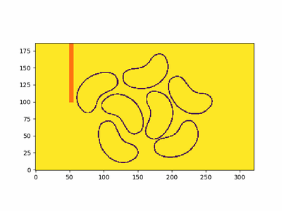
FSM performs computations in sweeps - and each sweep approximates the arrival time along one direction, and these are implicitly combined, as the sweeps happen one after the other. There are $2^2=4$ directions in a 2D domain. You can see it in action in the animation in Fig 1, with some bean-shaped initial fronts and an obstacle.

Now that you have some kind of intuition, let's understand the components of this algorithm.

1. Grid setup: As with any eulerian approximation, you divide your domain into a grid, with a grid spacing of choice. You identify the grid cells that you want the propagation to start from (source cells) and any obstacles in the way. Note that since these cells are marked as "frozen" - they do not participate in the computation. The algorithm basically skips these points.
2. You initialise the source points to have an arrival time of 0 - this will be fixed. All other points are initialised to a "large enough value"^[1]
3. In each sweep, you update the arrival time of the current cell based on values of the neighbouring cells. Here, we locally solve the Eikonal equation. The spatial derivative is approximated by a Godunov upwind difference scheme, which is sensitive to the direction of information flow, something crucial in this problem. Basically, if the "wave" is arriving from the bottom for example, it should mainly use values from these cells. You can read more about it here. It sounds like a fancy term, but it really isn't, and is quite simple to implement. Solving the Eikonal equation locally involves solving a quadratic equation (equation 2.4 in Zhao's paper).
4. Sweeps cover the $2^n$ (4 in 2D) combinations of coordinate directions, ensuring information propagating from all relative 'quadrants' (e.g., increasing x / increasing y, decreasing x / increasing y, etc.) is correctly captured by the upwind scheme. As mentioned earlier, the upwind scheme needs to respect the direction of information flow, and each of the 4 sweeps contribute information from a specific direction, which are all combined in the final algorithm.

Code #

There's only so much I can talk about it. To really understand it, do play with the code. I'll first show you the numpy code, which is easier to understand, before moving on to the JAX code. The JAX code is the same logic, but things are reorganised for efficiency with just in time compilation. What I like about these algorithms is that since interface propagation is such a visual problem, seeing their outputs and playing with the code can be really engaging. All the code is available in this repo, and you'll find this demo notebook a good place to start playing with it ^[2].

numpy #

import numpy as np


def fast_sweep_2d(grid, fixed_cells, obstacle, f, dh, iterations=5):
    # this is used for padding the outer boundaries of the domain,
    # so that the min() operations in the upwind scheme choose the inner point.
    large_val = 1e3
    nx, ny = grid.shape
    # 4 directions to sweep along - the range parameters for x and y.
    sweep_dirs = [
        (0, nx, 1, 0, ny, 1),  # Top-left to bottom-right
        (nx - 1, -1, -1, 0, ny, 1),  # Top-right to bottom-left
        (nx - 1, -1, -1, ny - 1, -1, -1),  # Bottom-right to top-left
        (0, nx, 1, ny - 1, -1, -1),  # Bottom-left to top-right
    ]

    # pad with a large value to properly handle boundary conditions in the upwind scheme.
    padded = np.pad(grid, pad_width=1, mode="constant", constant_values=large_val)

    for _ in range(iterations):
        for x_start, x_end, x_step, y_start, y_end, y_step in sweep_dirs:
            for iy in range(y_start, y_end, y_step):
                for ix in range(x_start, x_end, x_step):
                    # dont do anything for fixed cells (interface) or obstacles
                    if fixed_cells[iy, ix] or obstacle[iy, ix]:
                        continue
                    # calculate a,b from eqn 2.3 of Zhao et.al
                    py, px = iy + 1, ix + 1
                    # since it's a padded array and boundary+1 is a large value,
                    # it will choose the interior value at the end, acting like one sided difference.
                    a = np.min((padded[py, px - 1], padded[py, px + 1]))
                    b = np.min((padded[py - 1, px], padded[py + 1, px]))
                    # explicit unique solution to eq 2.3, given by eq 2.4
                    xbar = (
                        large_val  # xbar will be the distance to this cell from front
                    )
                    if np.abs(a - b) >= f * dh:
                        xbar = np.min((a, b)) + f * dh
                    else:
                        # can add small eps to sqrt later for stability
                        xbar = (a + b + np.sqrt(2 * (f * dh) ** 2 - (a - b) ** 2)) / 2
                    # update if new distance is smaller
                    padded[py, px] = np.min((padded[py, px], xbar))
    # return un-padded array
    return padded[1:-1, 1:-1]

You'd call it like this:

out = fast_sweep_2d(
    dist_grid_np,  # initial distance grid - 0 at interface, large val everywhere else
    interface_mask,  # 1 at interface, 0 elsewhere
    obstacle_mask,
    f=1,  # propagation speed
    dh=dh,  # grid spacing - is 1 for an image
    iterations=5,
)

jax #

And the code in JAX!

import jax
import jax.numpy as jnp
from functools import partial


@partial(jax.jit, static_argnames=["iterations"])
def fast_sweep_2d(grid, fixed_cells, obstacle, f, dh, iterations=5):
    large_val = 1e3
    nx, ny = grid.shape
    sweep_dirs = [
        (0, nx, 1, 0, ny, 1),  # Top-left to bottom-right
        (nx - 1, -1, -1, 0, ny, 1),  # Top-right to bottom-left
        (nx - 1, -1, -1, ny - 1, -1, -1),  # Bottom-right to top-left
        (0, nx, 1, ny - 1, -1, -1),  # Bottom-left to top-right
    ]
    frozen = jnp.logical_or(fixed_cells, obstacle)
    padded = jnp.pad(grid, pad_width=1, mode="constant", constant_values=large_val)

    def run_sweep(sweep_dir, grid):
        x_start, x_end, x_step, y_start, y_end, y_step = sweep_dir

        def y_loop_body(iy, grid):
            def x_loop_body(ix, grid):
                piy, pix = iy + 1, ix + 1
                a = jnp.minimum(grid[piy, pix - 1], grid[piy, pix + 1])
                b = jnp.minimum(grid[piy - 1, pix], grid[piy + 1, pix])
                updated_val = jnp.where(
                    frozen[iy, ix],
                    grid[piy, pix],  # no change if frozen
                    jnp.minimum(  # min of curr and updated val
                        grid[piy, pix],
                        jnp.where(  # eqn 2.4
                            jnp.abs(a - b) >= f * dh,
                            jnp.minimum(a, b) + f * dh,
                            (a + b + jnp.sqrt(2 * (f * dh) ** 2 - (a - b) ** 2)) / 2,
                        ),
                    ),
                )
                return grid.at[piy, pix].set(updated_val)

            x_indices = jnp.arange(x_start, x_end, x_step)
            return jax.lax.fori_loop(
                0,
                len(x_indices),
                # ix is 0..len(x_indices) - we need to map it to actual range
                lambda ix, grid: x_loop_body(x_indices[ix], grid),
                grid,
            )

        y_indices = jnp.arange(y_start, y_end, y_step)
        return jax.lax.fori_loop(
            0,
            len(y_indices),
            lambda iy, grid: y_loop_body(y_indices[iy], grid),
            grid,
        )

    def iteration_body(_, cur_grid):
        # perform 4 sweeps (2 dimentions)
        grid_s1 = run_sweep(sweep_dirs[0], cur_grid)
        grid_s2 = run_sweep(sweep_dirs[1], grid_s1)
        grid_s3 = run_sweep(sweep_dirs[2], grid_s2)
        grid_s4 = run_sweep(sweep_dirs[3], grid_s3)
        return grid_s4

    final_grid = jax.lax.fori_loop(0, iterations, iteration_body, padded)
    return final_grid[1:-1, 1:-1]

In action #

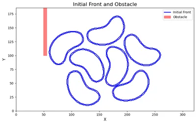
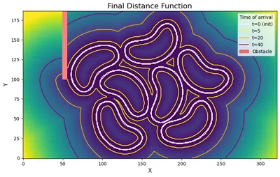
Here's an example of the fast sweeping method in action. We have some bean outlines (made here, heh), which I processed to be (greyscale) 0 at the boundary and 255 everywhere else. I've also added an obstacle (in red). We can see that it computes the distance function (not the signed distance function), by noticing the contours inside the beans for a $t=5$. If you want a SDF, the sign information needs to be available. For example, if we have a matrix of the same shape as the grid, with -1 inside the shape, 0 on the surface, and 1 outside, we could simply multiply this matrix with the distance function to get the signed distance function. I mention SDFs, as using FSM to generate SDFs is quite common. In this case, I have not computed the sign information, so I leave just the distance field below. We use contour lines to visualise the fronts at different time points.

Benchmarks #

I ran a few benchmarks on my Apple M2 Pro chip. We can see that the JAX compiled code on CPU is much faster than the numpy code, as expected. Do note the log scale used on the y-axis of this plot. I also compared this with a FMM library - skfmm. The logic in the library is written in C++, making it faster than both approaches discussed here. However, when working with custom FSM approaches for domain-specific problems, I'd trade the speed of skfmm for the ease of hackability and experimentation that I'd get with the python code any day. Of course, you might be comfortable hacking C++ code :)

A note on parallel FSM #

Actually, I tried to speed this up even more by parallelising this algorithm, as outlined in section 2.1 of the follow-up paper by Hongkai Zhao. There are other more complex parallel FSM implementations as well, but I didn't look into them for now. The idea in Zhao's follow up paper is to run the sweeps in parallel, then combine them all with an element wise minimum operation. This seems easy enough of a change, but with JAX specifically, I could not figure out a way to do this. The challenge was a classic JAX issue - the variables that define the shape of the computation cannot be traced. I was trying to vmap over the sweep directions, but since they form arguments for the arange function, which determine computation shape, I could not have these be traced values - and by definition vmap works with tracing it's input data. No kind of reorganisation of data/variables helped enable this. To the reader - If there's a hack around this issue, I'd love to know!!

References #

1. Level Set Methods and Fast Marching Methods : Evolving Interfaces in Computational Geometry, Fluid Mechanics, Computer Vision, and Materials Science
2. The Fast Sweeping Algorithm by Martin Cavarga
3. And other hyperlinks on this blog :D

• Previous: (KANs part 1) An introduction to B-splines